A Little Introduction to Neural Networks

If you're anything like me, you may have recently heard people talk about AI a bit more. Apparently there are one or two companies that have made some progress in the field.

While I consider myself technologically savvy enough to use a computer and save a PDF, I've mostly spend time with my mind wandering whenever the topic comes up of how machine learning and neural networks function.

Nowadays, that's not the healthiest attitude, and since we at Felix Research are rather actively engaged in the field of using and developing Artificial Intelligence solutions, it became time to learn a bit more.

The problem that I have repeatedly faced is that many of the explanations of how the more complex models work feel a bit like this guide to drawing an Owl,

which while technically correct, sort of leaves out some key details.

Understandably, the large commercial providers (and cough 'non-profit' organisations) don't particularly have an interest in writing a guide for how to compete with them.

I'm in the fortunate position of not having to do all of our coding anymore (and I think the team is quite glad that we have Dimitri on board as our Founding Engineer), but I believe that I should know as much as possible about the subject, since it's pretty core to our business. As I learn, I figured I'd share this, and some of our readers might find it a useful 101-guide or reminder.

Linear Predictions with ML Models

The simplest possible model is a linear regression that takes an input and predicts an output.

Using Torch as one of the classic foundations for model building, we can quite simply write such a model.

In this simplest example, we are trying to train the model to learn y = 2x. Not really worth building a neural network for, but this example shows the basic structure of a neural network:

We define the Input and Output data for testing, our X and Y values, MSE loss and stochastic gradient descent (SGD). This is the most basic form of a model.

In this type of model, we use a mean squared error loss function to calculate the "wrongness" of a model prediction, and then gradient descent over epochs to train the model to be... less wrong. Our learning rate defines the step size at which we conduct this gradient descent.

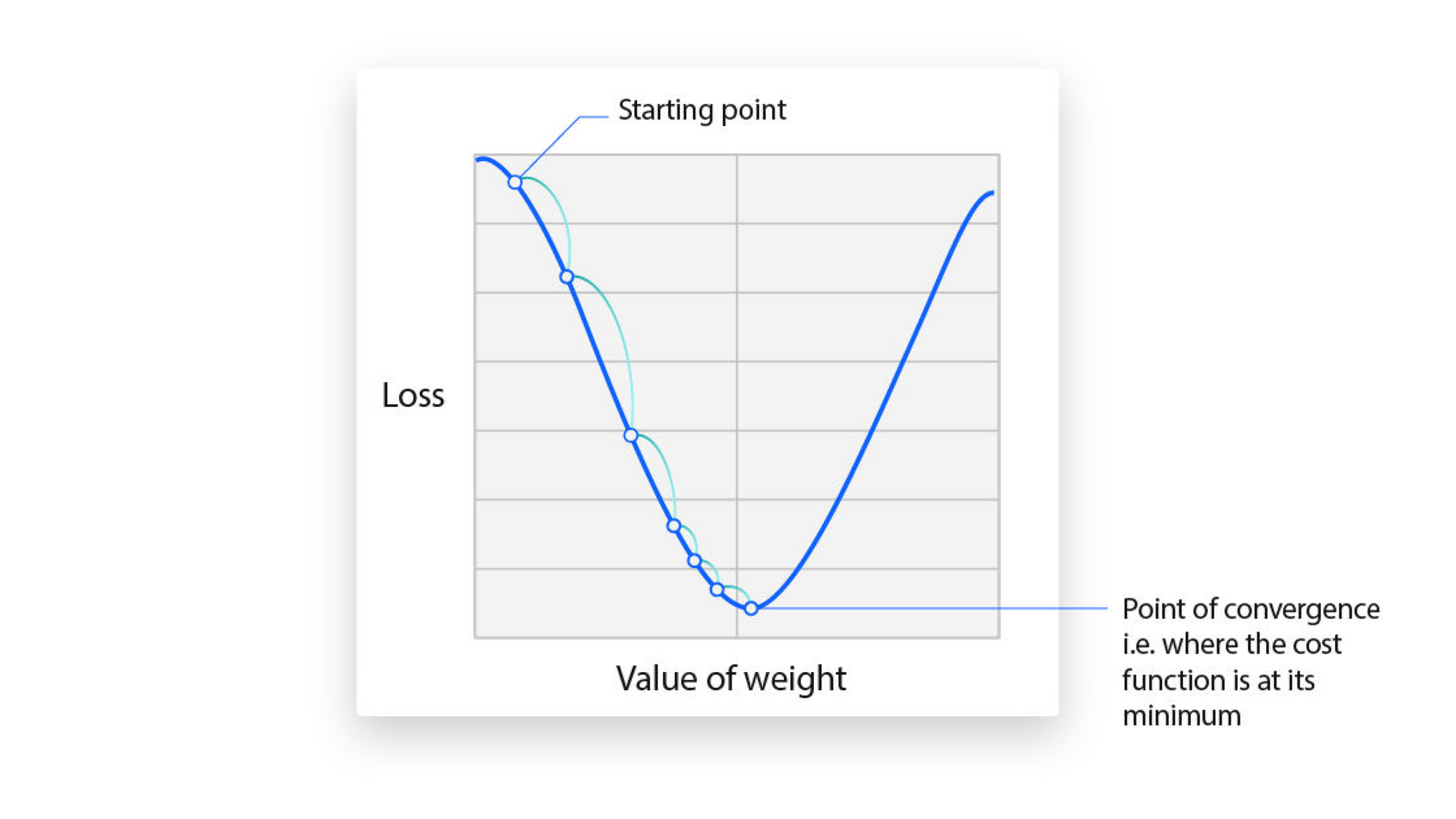
Changing our learning rate significantly impacts how and at what rate our weights get optimized to reduce loss, and involves a fair amount of trial and error.

The difference between gradient descent and stochastic gradient descent is primarily that in SGD we pick a random sample of our data at a given point in time rather than using the full sample of data to compute a gradient at each step, thus being more computationally efficient. [^1]

Important to note for the curious is that:

Strictly speaking, SGD was originally defined to update parameters by using exactly one training sample at a time. In modern usage, the term “SGD” is used loosely to mean “minibatch gradient descent,” a variant of GD in which small batches of training data are used at a time. The major advantage to using subsets of data rather than a singular sample is a lower noise level, because the gradient is equal to the average of losses from the minibatch. For this reason, minibatch gradient descent is the default in deep learning. Contrarily, strict SGD is rarely used in practice. These terms are even conflated by most machine learning libraries such as PyTorch and TensorFlow; optimizers are often called “SGD,” even though they typically use minibatches.

[^1] See IBM's great explainer on SGD for a better and more in depth explanation

import torch
import torch.nn as nn
import torch.optim as optim
import numpy as np

# 1. PREPARE DATA
# X is our input data, Y is our target data (labels).
# We must convert python lists into PyTorch Tensors.
X = torch.tensor([[1.0], [2.0], [3.0], [4.0], [5.0]], dtype=torch.float32)
Y = torch.tensor([[2.0], [4.0], [6.0], [8.0], [10.0]], dtype=torch.float32)

# 2. DEFINE THE MODEL
# We create a class that inherits from nn.Module
class SimpleNet(nn.Module):
    def __init__(self):
        super(SimpleNet, self).__init__()
        self.linear = nn.Linear(1, 1)

    def forward(self, x):
        return self.linear(x)

model = SimpleNet()

# 3. DEFINE LOSS AND OPTIMIZER
# Loss Function: Measures how wrong the model is.
# MSE (Mean Squared Error) is standard for regression.
criterion = nn.MSELoss()

# Optimizer: Updates the weights to reduce the error.
# SGD = Stochastic Gradient Descent. lr = learning rate.
optimizer = optim.SGD(model.parameters(), lr=0.01)

# 4. THE TRAINING LOOP
# This is the heart of AI programming.
# Adding history to let us inspect what happens
history = {
    'loss': [],
    'weight': [],
    'bias': []
}

epochs = 200
print("Training started...")

for epoch in range(epochs):
    # A. Forward pass: Compute predicted y by passing x to the model
    y_pred = model(X)

    # B. Compute loss: Difference between predicted and actual
    loss = criterion(y_pred, Y)
    
    # We use .item() to get the plain python number out of the Tensor
    history['loss'].append(loss.item())
    history['weight'].append(model.linear.weight.item())
    history['bias'].append(model.linear.bias.item())

    # C. Zero gradients: Clear old gradients before calculation
    optimizer.zero_grad()

    # D. Backward pass: Compute gradient of the loss with respect to model parameters
    loss.backward()

    # E. Step: Update parameters (weights) based on gradients
    optimizer.step()

    if (epoch+1) % 100 == 0:
        print(f'Epoch [{epoch+1}/{epochs}], Loss: {loss.item():.4f}')

checkpoint = {
    'model_state': model.state_dict(),
    'history': history
}

torch.save(checkpoint, "model_and_metrics.pth")
print("\nModel and metrics saved to model_and_metrics.pth")

This trains our most simple model that takes 1 input and 1 output over 200 epochs, and saves the model weights to a file, so we can load it again later.

Visually, we see graphs that may look familiar - as the training epochs go on, the MSE of the model decreases toward zero, and our weight and bias approach the actual mathematical function we are trying to imitate here.

In this case given the simplicity of the model, even a few epochs are enough to 'correctly' predict our output, but we do see that if we run the model at only 200 epochs, we are left with an output that is close, but given the equation, pretty far off the mark.

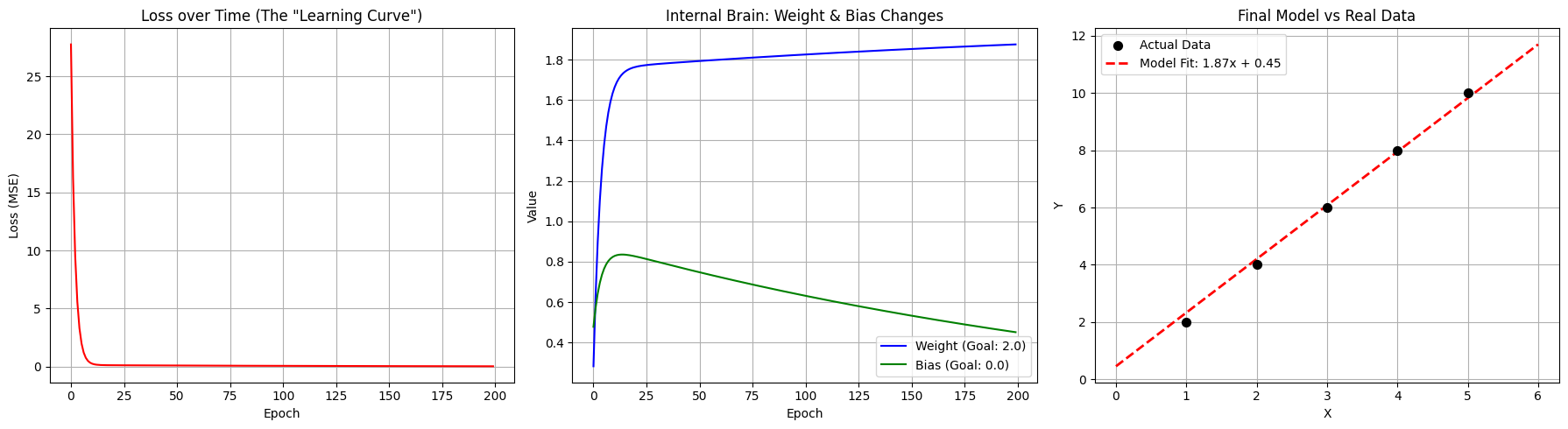
We can also train our model for a longer period, that is for more epochs, which... changes very little in this case, really.

Training started...
Epoch [100/100000], Loss: 0.0173
Epoch [200/100000], Loss: 0.0088
Epoch [300/100000], Loss: 0.0045
Epoch [400/100000], Loss: 0.0023
Epoch [500/100000], Loss: 0.0012
Epoch [600/100000], Loss: 0.0006
Epoch [700/100000], Loss: 0.0003
Epoch [800/100000], Loss: 0.0002
Epoch [900/100000], Loss: 0.0001
...
Epoch [100000/100000], Loss: 0.0000

Model and metrics saved to model_and_metrics.pth

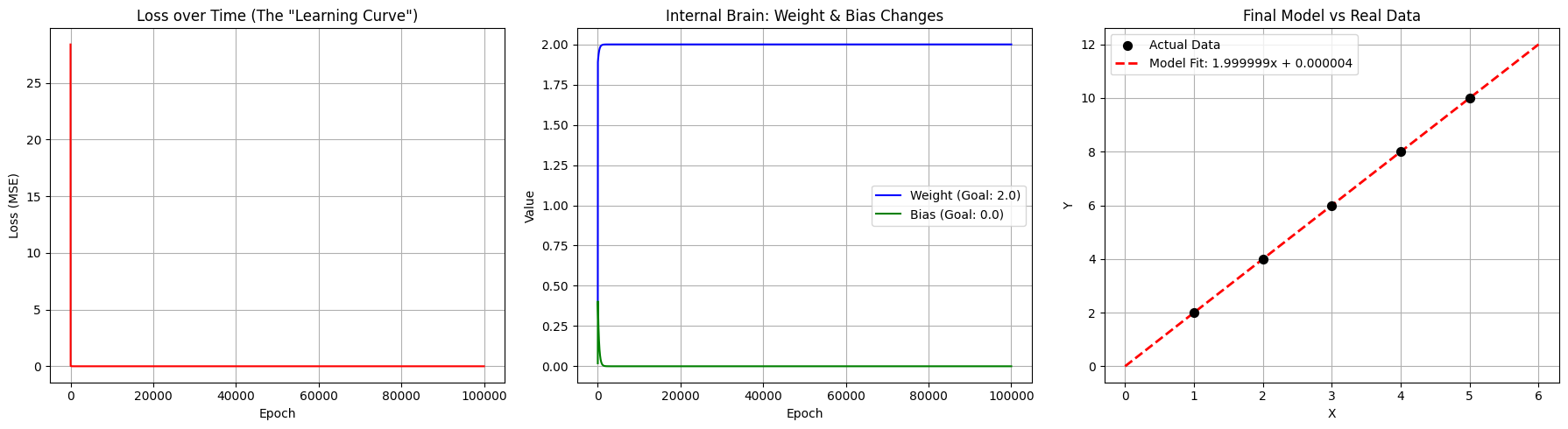
We are left with an essentially perfect model that predicts y = 2x, and we could now run this model to predict a value for this equation:

input_value = 20.0

# Convert the number into a Tensor of shape (1, 1)
input_tensor = torch.tensor([[input_value]])

# Turn off gradient calculation (saves memory/speed for inference)
with torch.no_grad():
    # Pass the tensor to the model
    prediction = model(input_tensor)

# Get the simple float value out of the resulting tensor
result = prediction.item()

print(f"Input: {input_value}")
print(f"Model Prediction: {result:.12f}")

Input: 20.0
Model Prediction: 39.999973297119

So What?

Now that we have wasted many orders of magnitude of compute beyond what's useful to predict that 20 * 2 in fact does equal 40 (or rather, failing to do so since we predict not quite 40), how do we make something that approaches a base level of usefulness?

ReLU

The above "model" is an example of linear regression, where we use the model to take an input and simply predict an output (Y = 2x + bias).

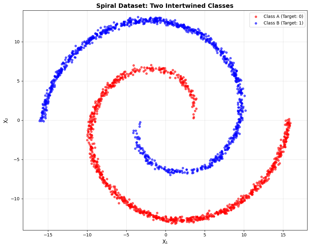
More use can be gotten from understanding how models can classify data, like a very simple example using colour. First, let's make a test set of data in the form of some spirals!

def create_spiral_data(n_points=1000):
    theta = np.sqrt(np.random.rand(n_points)) * 2 * np.pi 
    
    # Class A (Red) -> Target 0
    r_a = 2 * theta + np.pi
    data_a = np.array([np.cos(theta) * r_a, np.sin(theta) * r_a]).T
    x_a = data_a + np.random.randn(n_points, 2) * 0.2
    
    # Class B (Blue) -> Target 1
    r_b = -2 * theta - np.pi
    data_b = np.array([np.cos(theta) * r_b, np.sin(theta) * r_b]).T
    x_b = data_b + np.random.randn(n_points, 2) * 0.2

    # Combine
    X = np.vstack([x_a, x_b])
    # Labels: 0 for Class A, 1 for Class B
    Y = np.hstack([np.zeros(n_points), np.ones(n_points)])
    
    return torch.FloatTensor(X), torch.FloatTensor(Y).view(-1, 1)

X, Y = create_spiral_data()

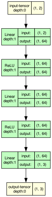
Let's use a new model, with an additional (and larger) layers to address the added complexity of our data, and supporting two inputs (our X and Y coordinates).

Importantly, we still output just one number, this being our probability (for the classification of red and blue dots)

class SpiralNet(nn.Module):
    def __init__(self):
        super(SpiralNet, self).__init__()
        self.layer1 = nn.Linear(2, 64)
        self.layer2 = nn.Linear(64, 64) 
        self.layer3 = nn.Linear(64, 1)  # Output is 1 number (Probability)
        self.relu = nn.ReLU()
        self.sigmoid = nn.Sigmoid() # Squishes output between 0 and 1

    def forward(self, x):
        x = self.relu(self.layer1(x))
        x = self.relu(self.layer2(x))
        x = self.sigmoid(self.layer3(x)) # Final activation for probability
        return x

model = SpiralNet()

We've added "ReLU" here, at which point I became scared of maths again and closed my computer.

When I returned, I put on my big boy pants and entered google, at which point I became scared again, since anything with more letters than numbers in maths is inherently scary, and that isn't helped when the second result starts with "A Gentle Introduction to..."

What are Rectified Linear Units?

Actually, quite simple!

ReLU(x) = max(0,x) where the output = input if the input is >= 0, and 0 otherwise.

Unlike linear functions like in the example above, where no transformation is applied at the cost of being unable to teach the model any complex functions, we can address this using ReLU, by being able to pass what appears to be a linear input to a model for backpropagation, since we receive the input for all values > 0, and 0 for those below, leaving us with a piecewise linear function.

The adoption of ReLU around 2010-11 is one of the significant milestones that has enabled significant progress in the deep learning field. Before its use, the primary methods used were logistic sigmoid and hyperbolic tangent functions, with both have problems with saturation.

See the excellent Gentle Introduction for mode detail on these.

A general problem with both the sigmoid and tanh functions is that they saturate. This means that large values snap to 1.0 and small values snap to -1 or 0 for tanh and sigmoid respectively. Further, the functions are only really sensitive to changes around their mid-point of their input, such as 0.5 for sigmoid and 0.0 for tanh.

We now set the loss criterion. In our Linear function, this was a Mean Squared Error loss, which works well for regression tasks.

For classification, like in our example, we want to use a loss function that maximises the penalty for incorrect guesses, which leads to better training results than a MSE-based version, where we consider the distance to a correct guess.

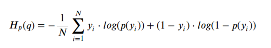
Cross Entropy Loss is more commonly used in these classification problems, as it measures the divergence between the predicted probability distribution and the true distribution of target classes.

If you're a mathematician, it looks like this:

If you're a programmer using the torch library, it looks like this:

import torch.nn as nn
nn.BCELoss()

# We changed MSELoss -> BCELoss (Binary Cross Entropy)
# This is used for Yes/No (1/0) classification questions
criterion = nn.BCELoss()
optimizer = optim.Adam(model.parameters(), lr=0.01)

# 4. TRAINING LOOP
# Adding history to track loss and accuracy over time
history = {
    'loss': [],
    'accuracy': []
}

epochs = 10000
print("Training on Spiral Data...")

for epoch in range(epochs):
    y_pred = model(X)
    loss = criterion(y_pred, Y)
    
    # Calculate accuracy (How many did we get right?)
    predicted_classes = y_pred.round() # Round to 0 or 1
    acc = (predicted_classes.eq(Y).sum() / float(Y.shape[0])).item()
    
    # Track history
    history['loss'].append(loss.item())
    history['accuracy'].append(acc)
    
    optimizer.zero_grad()
    loss.backward()
    optimizer.step()
    
    if (epoch+1) % 200 == 0:
        print(f'Epoch [{epoch+1}/{epochs}], Loss: {loss.item():.4f}, Accuracy: {acc*100:.2f}%')

# Save model state and history
checkpoint = {
    'model_state': model.state_dict(),
    'history': history
}
torch.save(checkpoint, "spiral_model.pth")
print("Model and metrics saved to spiral_model.pth")

After training our model, we can load the spiral again, and see that we have a red and a blue region respectively, showing the model's mapping of the space after it has been trained. In this dataset with clear space and separation between the two spirals, the model has very few regions in which it cannot confidently separate the red and blue regions.

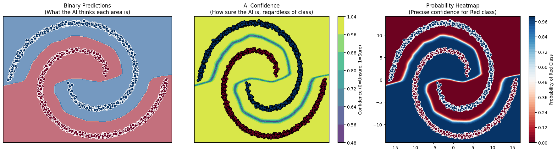
However, looking at the generated outputs and boundaries, it's clear that the model we have built here does not actually know what's 'red' or 'blue', it just splits the space into those two regions, leaving us with areas that are, visually, quite clearly outside the region of either spiral, and yet the model predicts with high confidence that this is a 'blue' or 'red' region respectively.

We can train the model with a third spiral, to separate the space further.

# 1. CREATE 3-CLASS SPIRAL DATA
def create_spiral_data(n_points=1000, classes=3):
    X = []
    y = []
    for i in range(classes):
        theta = np.sqrt(np.random.rand(n_points)) * 2 * np.pi 
        r = 2 * theta + np.pi
        
        # Rotate the spiral based on the class index
        # Class 0: 0 deg, Class 1: 120 deg, Class 2: 240 deg
        rotation = i * (2 * np.pi / classes)
        
        # Math to generate the spiral arms
        d = np.array([np.cos(theta) * r, np.sin(theta) * r]).T
        
        # Apply rotation matrix
        rot_mat = np.array([[np.cos(rotation), -np.sin(rotation)],
                            [np.sin(rotation), np.cos(rotation)]])
        d = np.dot(d, rot_mat)
        
        # Add noise
        d += np.random.randn(n_points, 2) * 0.2
        
        X.append(d)
        y.append(np.zeros(n_points) + i) # Label is 0, 1, or 2

    X = np.concatenate(X)
    y = np.concatenate(y)
    
    # Note: CrossEntropyLoss expects LongTensor for labels (integers), not Float
    return torch.FloatTensor(X), torch.LongTensor(y)

X, Y = create_spiral_data(classes=3)

# 2. DEFINE THE MODEL
class MultiSpiralNet(nn.Module):
    def __init__(self):
        super(MultiSpiralNet, self).__init__()
        self.layer1 = nn.Linear(2, 64)
        self.layer2 = nn.Linear(64, 64)
        # OUTPUT CHANGE: We now have 3 output neurons!
        # [Score for Class 0, Score for Class 1, Score for Class 2]
        self.layer3 = nn.Linear(64, 3) 
        self.relu = nn.ReLU()
        
        # Note: We do NOT put Softmax here. 
        # PyTorch's CrossEntropyLoss includes Softmax automatically for numerical stability.

    def forward(self, x):
        x = self.relu(self.layer1(x))
        x = self.relu(self.layer2(x))
        x = self.layer3(x) 
        return x

model = MultiSpiralNet()

# 3. LOSS (The "Big Gun" of AI)
criterion = nn.CrossEntropyLoss()
optimizer = optim.Adam(model.parameters(), lr=0.01)

# 4. TRAINING
epochs = 2000
print("Training 3-Class Spiral...")

for epoch in range(epochs):
    # Forward
    logits = model(X) 
    
    # Loss
    loss = criterion(logits, Y)
    
    # Backward
    optimizer.zero_grad()
    loss.backward()
    optimizer.step()
    
    if (epoch+1) % 200 == 0:
        # Calculate accuracy
        # torch.max returns (max_value, index_of_max_value)
        # We want the index (0, 1, or 2)
        _, predicted = torch.max(logits, 1)
        acc = (predicted == Y).sum().item() / Y.size(0)
        print(f'Epoch [{epoch+1}/{epochs}], Loss: {loss.item():.4f}, Accuracy: {acc*100:.2f}%')

torch.save(model.state_dict(), "spiral_3class.pth")
print("Model saved.")

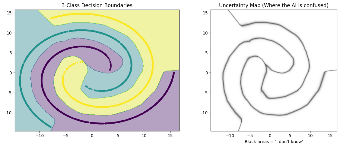
This leaves us with regions that are closer to the actual spiral areas, but this shows us what this model does, and importantly, what it does not do.

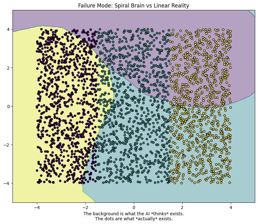
We want the neural networks we build to be useful. The small model that we have put together above is useful, but only for this one specific task.

Rather than the model actually recognizing red / blue / neither, it essentially builds a map of our space, predicting the likelyhood of any of the options appearing in that space.

We can visualise this by changing the input from a spiral, where we can see quite clearly that we have not built a model good at differentiating colour, but one that learns a space.

As we can see with the test data below where instead of a spiral, we generate a set of lines of coloured data, the model is entirely useless for this task. If we wanted the model to be able to classify these arrangements, we would have to train it again.

What's next?

In order to proceed beyond simple classification or simple prediction, as we have looked at in this brief overview post, we have to start talking about Convolutional Neural Networks, which can begin to use training data, like the classical MNIST example set, to understand handwritten numbers.

What is a CNN?

From Wikipedia:

CNNs are also known as shift invariant or space invariant artificial neural networks, based on the shared-weight architecture of the convolution kernels or filters that slide along input features and provide translation-equivariant responses known as feature maps. Counter-intuitively, most convolutional neural networks are not invariant to translation, due to the downsampling operation they apply to the input.
Feedforward neural networks are usually fully connected networks, that is, each neuron in one layer is connected to all neurons in the next layer. The "full connectivity" of these networks makes them prone to overfitting data. Typical ways of regularization, or preventing overfitting, include: penalizing parameters during training (such as weight decay) or trimming connectivity (skipped connections, dropout, etc.) Robust datasets also increase the probability that CNNs will learn the generalized principles that characterize a given dataset rather than the biases of a poorly-populated set.
Convolutional networks were inspired by biological processes in that the connectivity pattern between neurons resembles the organization of the animal visual cortex. Individual cortical neurons respond to stimuli only in a restricted region of the visual field known as the receptive field. The receptive fields of different neurons partially overlap such that they cover the entire visual field.

Essentially, in a CNN, the input is broken into kernels. For example, in the model we set up below, we take a 28x28 pixel image, and break it into 3x3 kernels. The model then extracts a set of "features" from the images that it learns over epochs of training.

Importantly, as you are no doubt aware, when anyone talks about model responses, these are always, ultimately, a probability expression of the most likely answer out of the possible options.

At the end of our model, we have a layer with 10 outputs (numbers 0-9), which we flatten (with ReLU), to arrive at the activation of the layer that corresponds to our number value, which is the final model response.

In a dataset like the MNIST training set, we train the model with a large amount of test data, where each test image is labelled with its corresponding number. The model here effectively learns what shapes correspond to what labelled number, so that when we ask it to identify a number after training, it can identify the closest likely matching number.

import torch
import torch.nn as nn
import torch.optim as optim
from torchvision import datasets, transforms
from torch.utils.data import DataLoader

# 1. PREPARE DATA (MNIST)
# Transforms allow us to turn raw images into Tensors
transform = transforms.Compose([
    transforms.ToTensor(),
    transforms.Normalize((0.1307,), (0.3081,)) # Standard normalization for MNIST
])

# Download data
train_dataset = datasets.MNIST('./data', train=True, download=True, transform=transform)
# DataLoader handles batching (giving us 64 images at a time)
train_loader = DataLoader(train_dataset, batch_size=64, shuffle=True)

# 2. DEFINE THE CNN MODEL
class SimpleCNN(nn.Module):
    def __init__(self):
        super(SimpleCNN, self).__init__()
        
        # --- FEATURE EXTRACTION (The "Eyes") ---
        # Layer 1: Input 1 channel (grayscale) -> Output 32 features
        # Kernel 3x3 means it looks at small 3x3 squares
        self.conv1 = nn.Conv2d(in_channels=1, out_channels=32, kernel_size=3, padding=1)
        
        # Layer 2: Input 32 features -> Output 64 features
        self.conv2 = nn.Conv2d(in_channels=32, out_channels=64, kernel_size=3, padding=1)
        
        # Pooling: Shrinks image by half (2x2)
        self.pool = nn.MaxPool2d(kernel_size=2, stride=2)
        
        # --- DECISION MAKING (The "Brain") ---
        # We need to calculate the size of the flattened input.
        # MNIST is 28x28. 
        # After Pool 1 (28->14). After Pool 2 (14->7).
        # Final Grid is 7x7 pixels. We have 64 feature maps.
        # So: 64 * 7 * 7 = 3136 inputs.
        self.fc1 = nn.Linear(64 * 7 * 7, 128)
        self.fc2 = nn.Linear(128, 10) # 10 Outputs (Digits 0-9)
        
        self.relu = nn.ReLU()
        self.flatten = nn.Flatten()

    def forward(self, x):
        # Pass 1: Conv -> ReLU -> Pool
        # Input: [Batch, 1, 28, 28] -> Output: [Batch, 32, 14, 14]
        x = self.pool(self.relu(self.conv1(x)))
        
        # Pass 2: Conv -> ReLU -> Pool
        # Input: [Batch, 32, 14, 14] -> Output: [Batch, 64, 7, 7]
        x = self.pool(self.relu(self.conv2(x)))
        
        # Flatten: Turn Grid into Line
        # Output: [Batch, 3136]
        x = self.flatten(x)
        
        # Classification
        x = self.relu(self.fc1(x))
        x = self.fc2(x)
        return x

model = SimpleCNN()

# 3. LOSS & OPTIMIZER
criterion = nn.CrossEntropyLoss()
optimizer = optim.Adam(model.parameters(), lr=0.001)

# 4. TRAIN
print("Training CNN on MNIST digits...")
epochs = 3 # CNNs learn FAST. 3 epochs is enough for >98% accuracy.

for epoch in range(epochs):
    running_loss = 0.0
    for batch_idx, (data, target) in enumerate(train_loader):
        # Standard training steps
        optimizer.zero_grad()
        output = model(data)
        loss = criterion(output, target)
        loss.backward()
        optimizer.step()
        
        running_loss += loss.item()
        
        if batch_idx % 100 == 0:
            print(f'Epoch {epoch+1}, Batch {batch_idx}: Loss {loss.item():.4f}')

print("Training Complete.")
torch.save(model.state_dict(), "mnist_cnn.pth")

When we run this model, training takes quite a bit longer to train than the previous little testers we've built, as a result of the added complexity of our model and its layers.

We can see the difference in structure between the simple model we built for our spirals

and the MNIST training model

What can this model do? The MNIST training model is a sort of classic learning piece, which lets us recognize handwritten numbers from their training set, for example we can load one of the test images for the number '1', and indeed

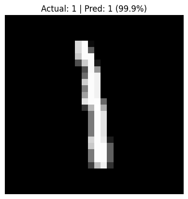
The model correctly and confidently predicted our number.

Neat.

What now?

None of the above is new, but by going through the stages of models to this point logically, and beginning to understand some of the choices that are made to achieve the desired results, it helps us to be able to speak the language of neural networks, and to begin playing around with more complex cases. We went from a simple linear model all the way to a basic convolutional neural network, from predicting y = 2x to recognizing handwritten numbers.